LiDAR → Utility Network → Metadata, End-to-End

01The question

Can free public LiDAR replace paid utility survey flights?

Paid survey flights return 20 to 190 points per m², priced per line mile. USGS 3DEP is free and covers most of the US, but at 2 to 8 points per m².

Raw LiDAR return intensity over a utility corridor — Return intensity per point.

The same corridor, segmented into poles, wires, ground and vegetation — Poles, wires, ground, vegetation.

02The problem

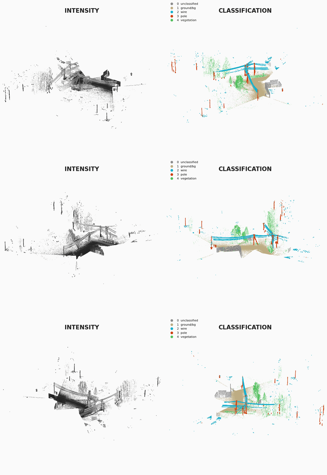
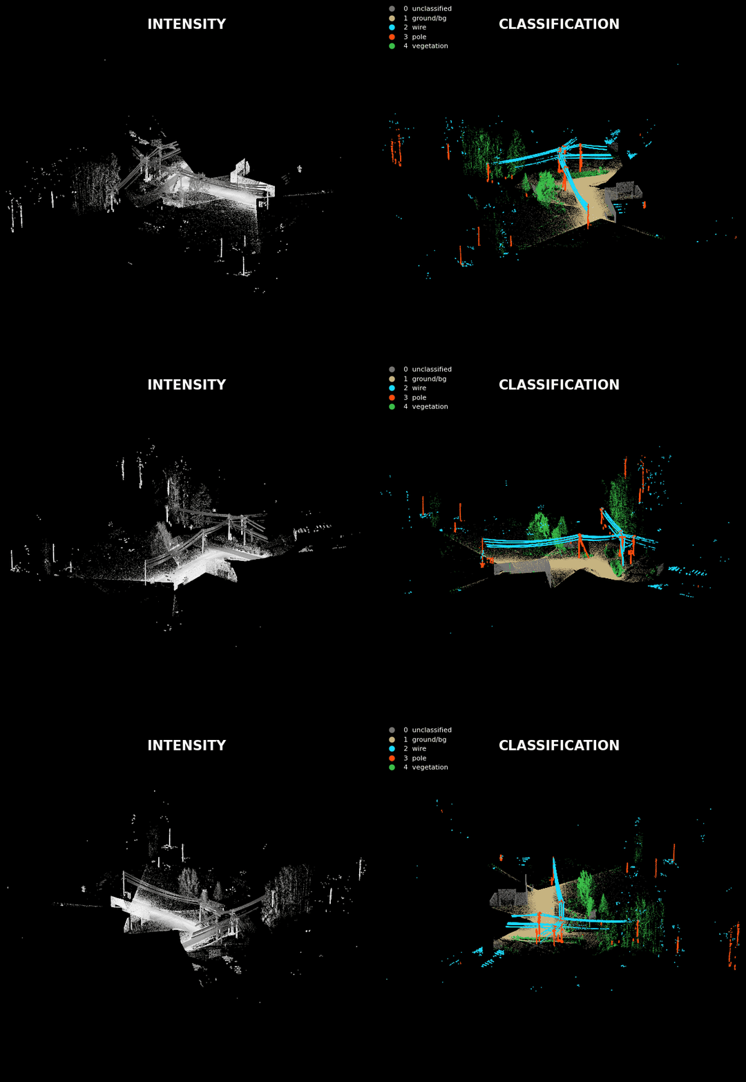
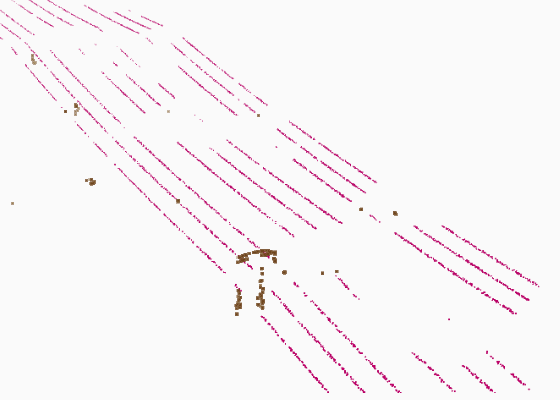
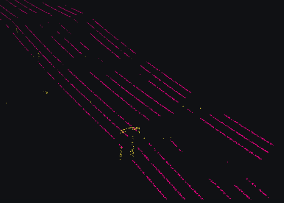
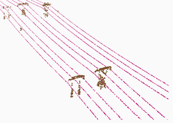
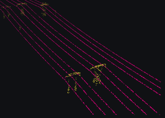
Thin a scan ten times and ground and trees keep their shape, but wires become scattered points and poles a smudge. The classes that matter fail first, and a model validated at survey density never sees it happen. Scores below are IoU, the overlap between prediction and truth, where 1 is perfect.

Same tile at 5 points per square metre, model trained at full density only: wires break up, poles vanish — 5 pts/m²: wires break, poles vanish.

wire IoU 0.58pole IoU 0.42

Same tile at 5 points per square metre, model trained across densities: wires and poles intact — Same tile: wires and poles hold.

wire IoU 0.95pole IoU 0.65

at full density both scorewire IoU 0.96pole IoU 0.71

03What I built

LiDAR
segmentation
topology
wire separation
metadata

Segmentation that survives sparsity

Every training tile is also thinned to 12, 8 and 5 points per m², so the model sees sparse data from the start. A large frozen encoder is gated into a small trainable backbone, adding its knowledge at no inference cost.

LitePT 13M trainable frozen PTv3 124M Pointcept checkpointmulti-density corpusrare-class loss

Topology in one forward pass

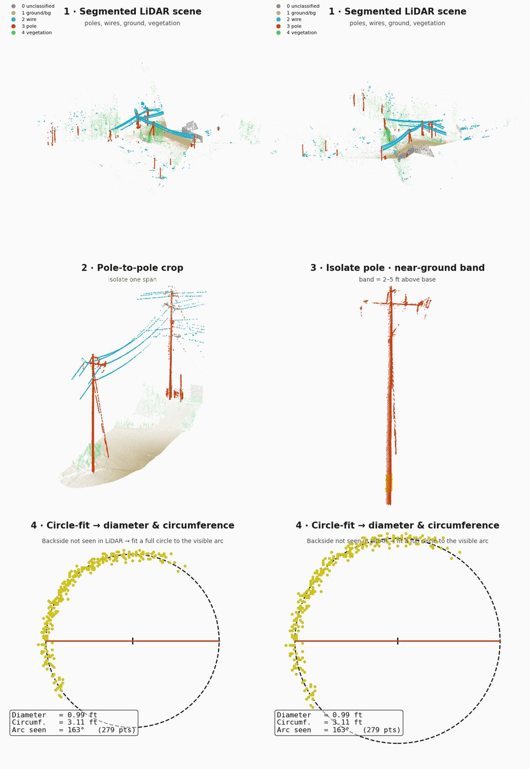
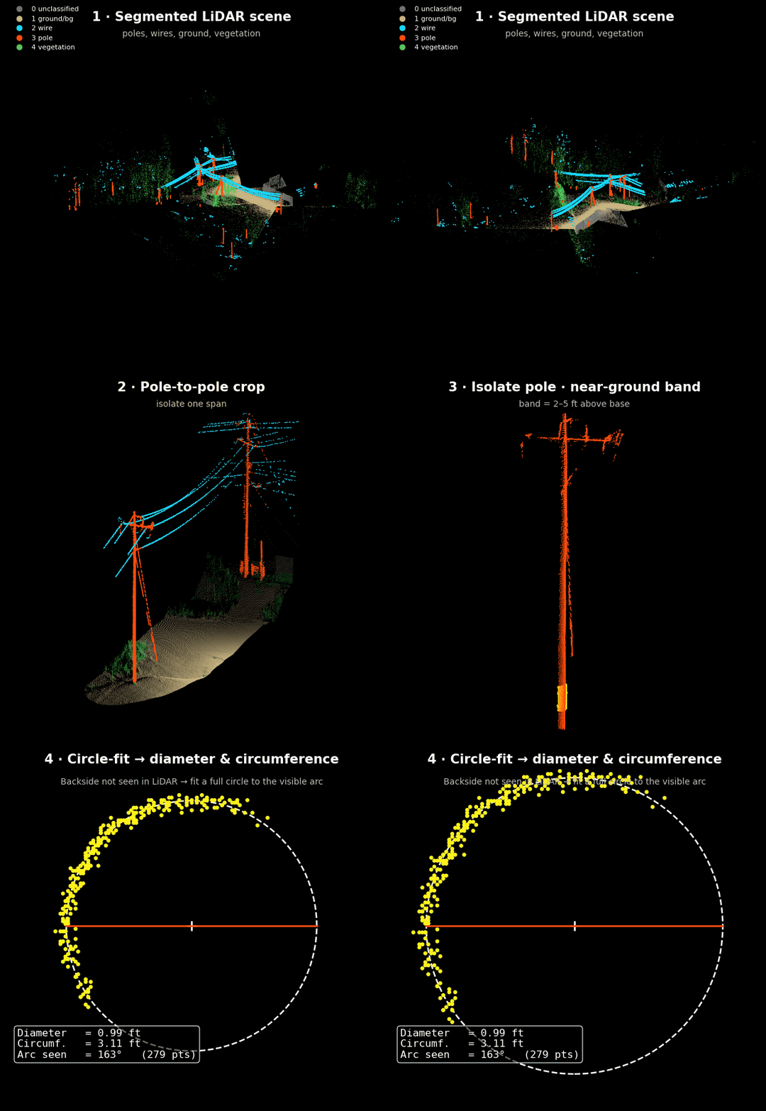
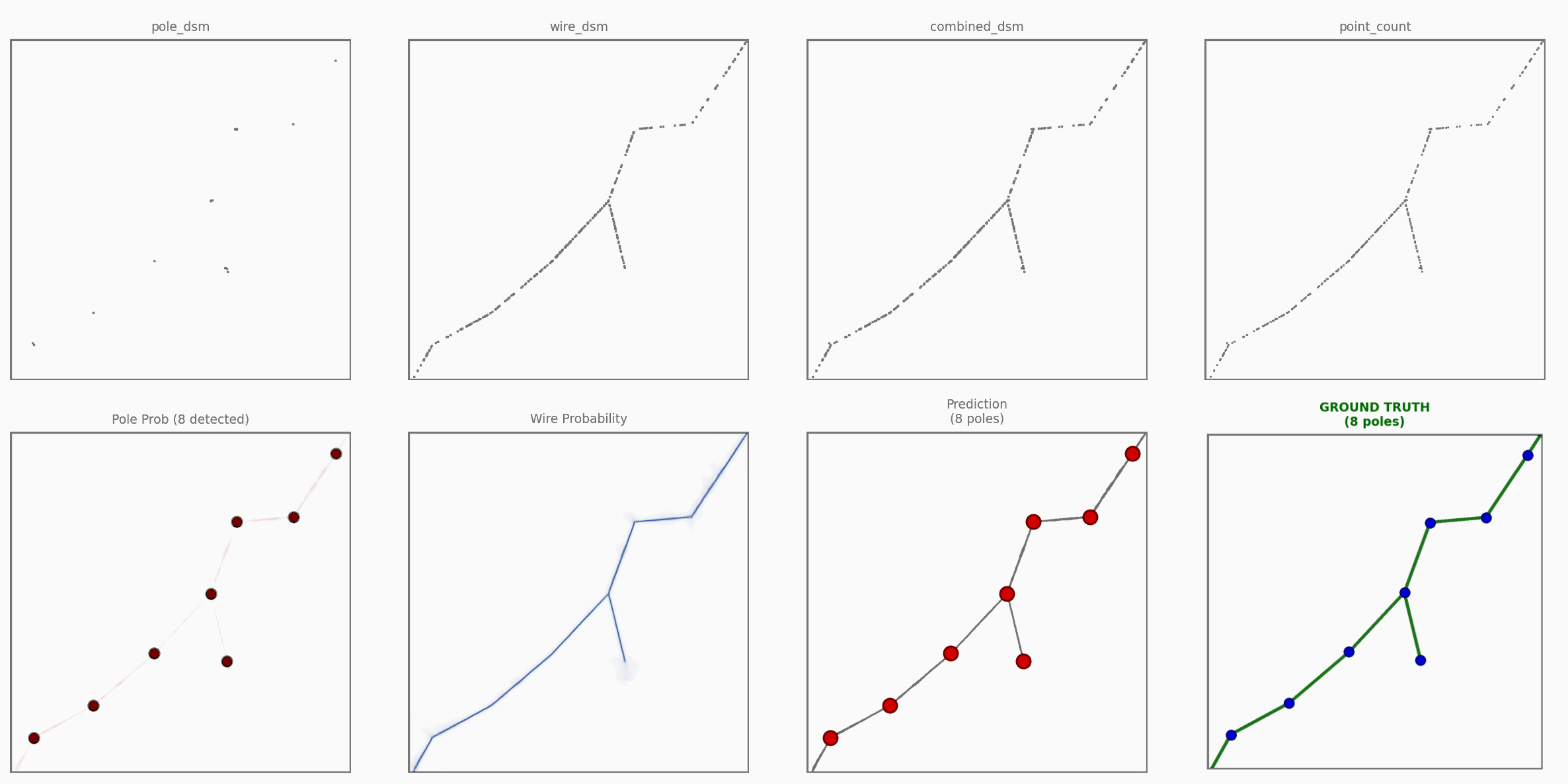
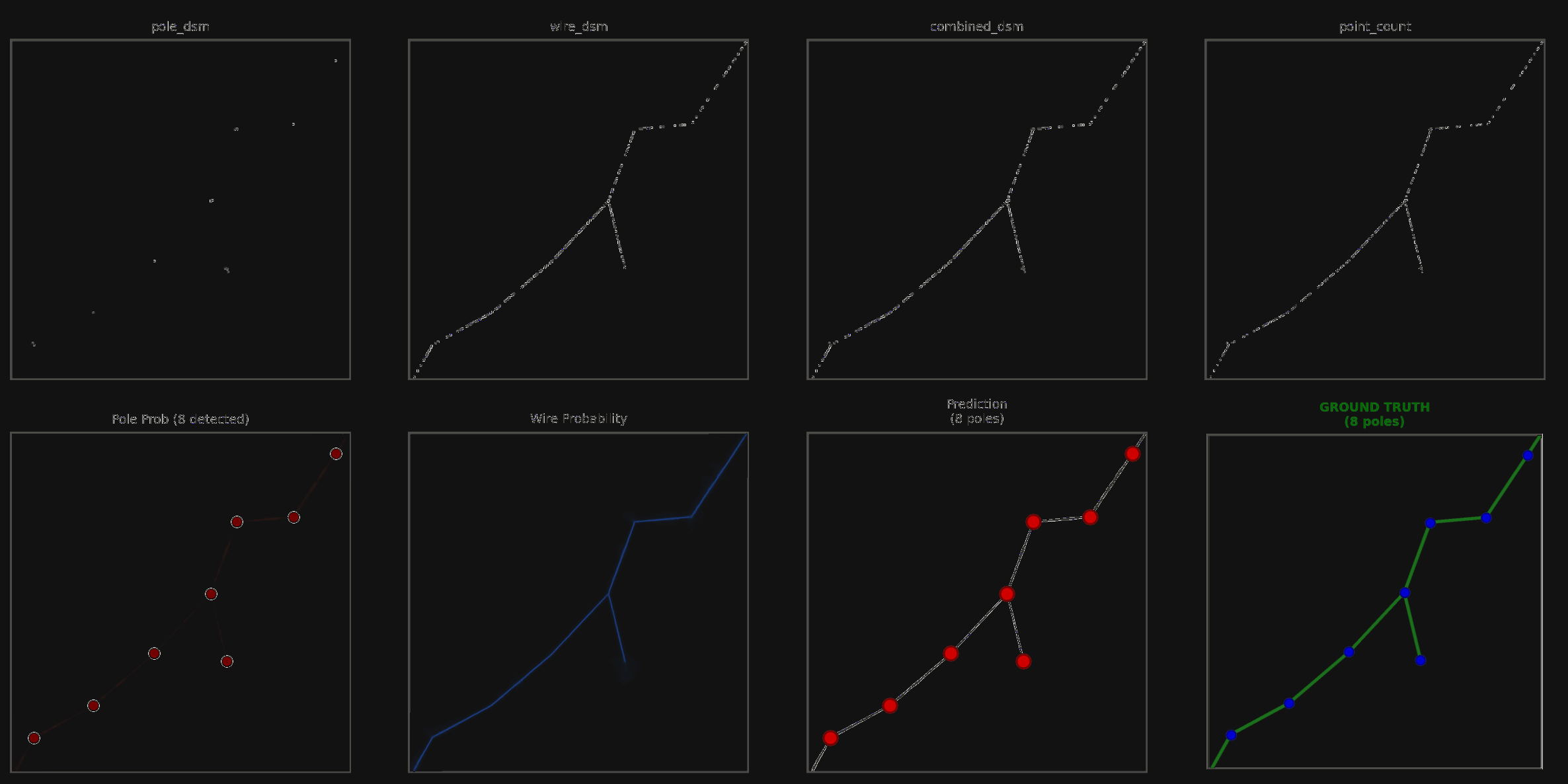
A four-channel height map feeds a dual-head network that predicts poles and wires together in one pass. The channels that depend on point labels are dropped at random in training, so the network still works when a scan is badly classified.

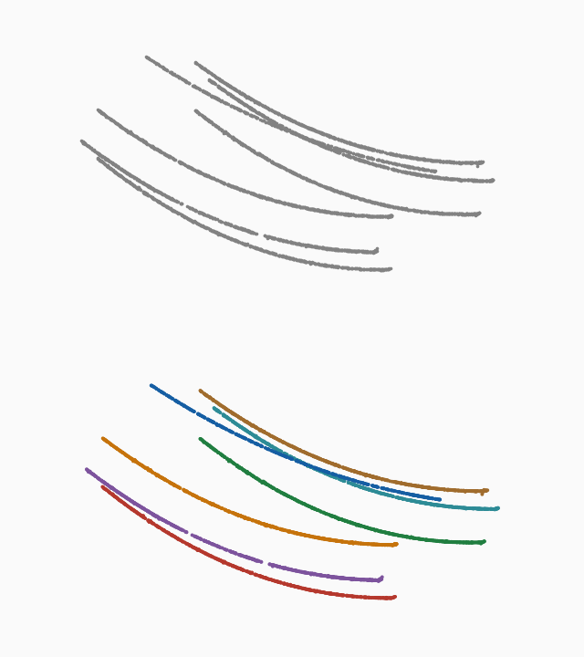
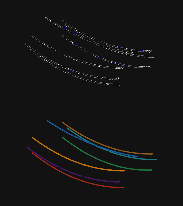
4-channel DSM ResUNet FPNdual headchannel dropoutclDice lossglobal span assembly

One span → individual conductors

A learned separator and a geometric one fail in opposite situations, so a gate picks the better one per span. A catenary curve is then fitted to each conductor.

PointNet on synthetic spans PCAcatenary straighteningHDBSCAN mixture-of-experts gate

A span of seven transmission wires: raw above, separated into one colour per wire below — Raw, then per wire.

Metadata, one record per asset

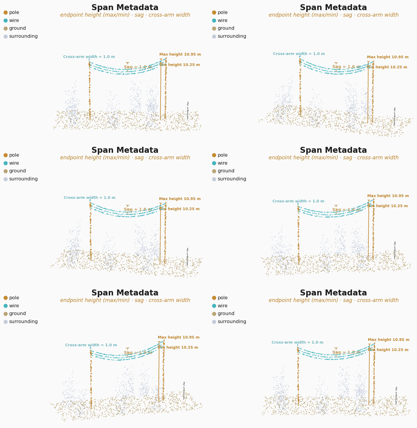
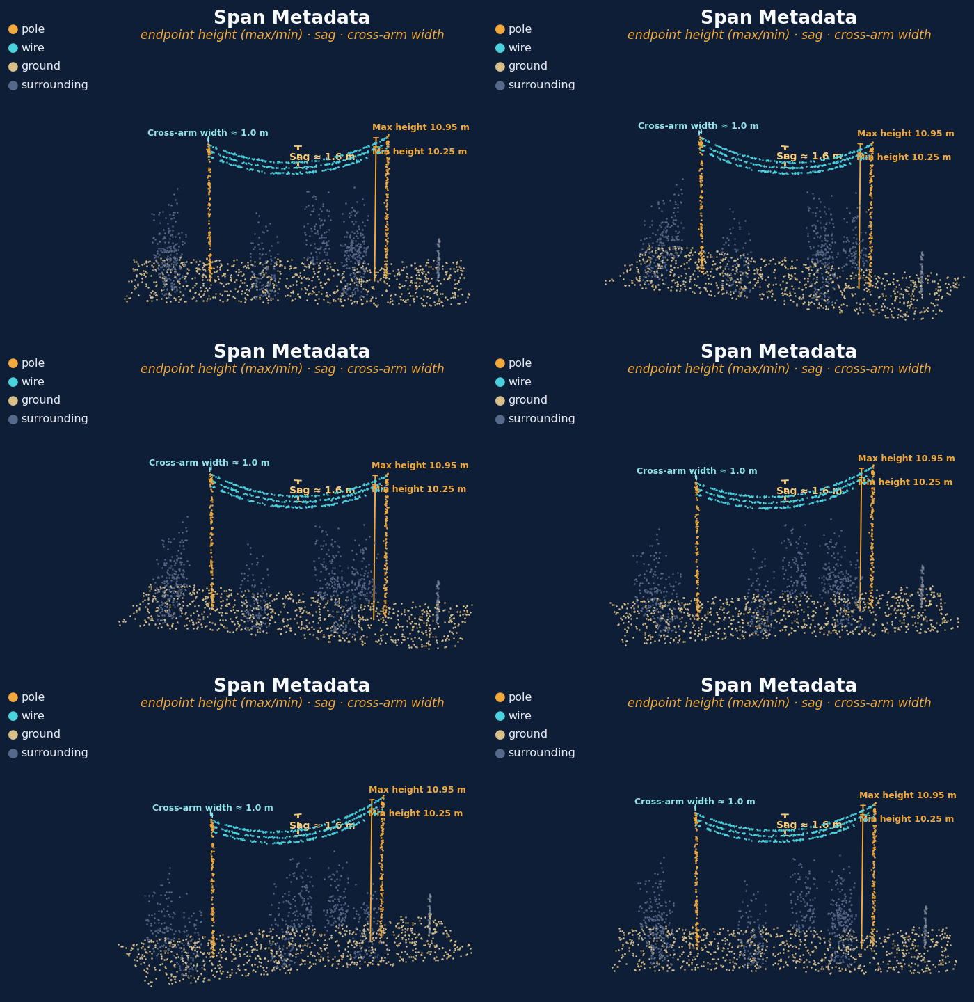
With every conductor a fitted curve, the record writes itself: wire endpoints, pole heights and vegetation clearance. Clearance is the number that tells a utility where to trim before fire season.

wire endpoints and sagpole height and locationground clearancevegetation clearance

04Results

Segmentation

	wire IoU	pole IoU
USGS 3DEP, real scans at 3.5 pts/m²	0.10 → 0.84	0.30 → 0.84
DALES	0.86 → 0.96	0.47 → 0.72
ECLAIR, never seen in training	0.88 → 0.98	0.16 → 0.74
Toronto-3D, never seen in training	0.56 → 0.61	0.49 → 0.61

Pre-trained Point Transformer V3 (Pointcept), used as is → ours. Open datasets, one protocol, no retraining.

Network

≥ 0.91pole detection, 0.4 to 193 pts/m², clean to badly classified
99.8%precision assigning points to individual conductors

Poles become nodes and spans become edges, assembled across tiles so a span that crosses a tile boundary is still one edge.

Top row: the four DSM input channels for one tile. Bottom row: pole probability, wire probability, the predicted graph with eight poles, and the ground truth with eight poles — One tile: input channels, pole and wire heatmaps, predicted graph, ground truth. Eight poles in, eight out.

Metadata

12–18 cmerror on conductor endpoint height and sag

Every conductor is a fitted curve through real returns, so each measurement is a simple query on the curve. Vegetation clearance is the number that decides where a wildfire can start.

One span with its measured endpoint heights, sag and cross-arm width — One span, measured.

05In production

normalise
segment
clip spans
topology
polygonise
metadata

Live in production. Six scale-to-zero endpoints, each on the instance type it needs, so shipping a new model is a configuration change.

AWS SageMakerCPU / GPU splitTerraform MLflow model aliases

06Impact

500K+line miles · US, Canada, Europe · public, customer-flown and mobile LiDAR
50K+line miles in a single job

Per-span vegetation clearance shipped as a product: where to trim before fire season.
64 percent of one utility’s GIS spans recovered from public LiDAR alone.
Next: where no LiDAR was ever flown, teach a depth model the canopy heights this pipeline already produces, so imagery alone can fill the gaps.